Intent Embeddings for Daisy ESP32 Badge
- Embedded , Gen ai , Ml
- December 2, 2025
This is the 4th Blog in our series about building an AI-powered conference badge on the ESP32-S3. In the previous blog, we got our custom “Hey Daisy” wake word somewhat working. Now the badge can listen for its trigger phrase. But what happens after it hears “Hey Daisy”?
The original plan was simple: Wake word triggers recording, recording goes to Speech-to-Text, transcribed text feeds into the LLM. Clean, elegant, and completely impossible on our hardware. hehe right, its impossible to fit a full vocab SST into that tiny thing (tho I intent to try in a version 2)
This is the story of how a dead end led to something over-engineered and interesting.
Well STT Died
I had this beautiful mental model of how voice interaction would work. User says “Hey Daisy,” badge starts recording, audio gets transcribed to text, text gets processed by the LLM, response gets spoken back. Just like every smart speaker you’ve ever used.
The problem? Smart speakers have cloud backends. We have 8MB of PSRAM. (Its a hard requirement I kept on myself to NOT use any external service and run everything locally. Whats the fun in just calling API services, I found running everything on this tiny thing a very nice challenge.)
Let me share a rough math:
| Model | Size | Notes |
|---|---|---|
| Whisper Tiny | ~75MB | Smallest official Whisper |
| Whisper Tiny.en (INT8) | ~39MB | Quantized, English-only |
| wav2vec 2.0 | ~100MB+ | Facebook’s model |
| DeepSpeech | ~180MB | Mozilla’s attempt |
| Vosk (small) | ~50MB | Supposedly “lightweight” |
Our constraint: 8MB PSRAM total. I simply couldn’t find an STT model that would fit. (Maybe I should have trained one, it did not cross my mind at the moment to train a STT model from scratch, the tiniest model looked quite large so I didn’t wanna even try I guess)
I spent an embarrassing amount of time looking for The Magical Tiny STT Model that surely existed somewhere. I searched through every Tiny repository, every quantization paper, every pruning technique. The answer was always the same: speech recognition requires representing the acoustic space of human language, and that space is fundamentally large. What a bummer!
The architecture I’d been planning assumed STT would work. Without it, how would the LLM know what the user asked? The obvious fallback was push-button interaction with a text interface. Type your question, get a response. But that defeats the entire point of a voice-activated badge. Conference attendees shouldn’t need to pull out their phones to interact with a novelty item.
I was staring at my dataset - 2,008 questions about myself that the LLM was trained to answer - when the idea hit me.
Intent Similarity
So hold your beers and think, I have 2k known questions. Why do I need to transcribe the audio at all?
Think about it. Speech-to-Text is general-purpose - it can transcribe anything you say into text. But I don’t need “anything.” I need to figure out which of my 2k questions the user just asked. This isn’t transcription. This is classification. Or more precisely, it’s similarity matching.
The idea:
- Pre-compute text embeddings for all 2k questions (stored on SD card)
- Record user’s spoken question
- Generate an audio embedding from the recording
- Find the closest text embedding using cosine similarity
- Pass that matched question to the LLM, easy peasy! (If not close enough, I can make llm say I don’t know or something generic like that)
We’re trading flexibility for efficiency. A traditional STT system could transcribe “Tell me about your favorite debugging story from 2019” even if that exact phrase isn’t in our database. Our approach can only match to known and similar questions, if I had time I would have even built a online self-retraining flow that would update the model based on similarity score. (I honestly did sketch that up as well in my figjam board)
The Architecture
The system has two branches that need to produce compatible embeddings:
Audio Branch (runs on ESP32): Raw Audio (16kHz) → Mel-Spectrogram (64×96) → CNN Encoder → 256-dim embedding
Text Branch (runs once during training): Question Text → MPNet (768-dim) → Projection Layer → 256-dim embedding
The idea here is that both branches output vectors in the same 256-dimensional space. If the audio and text represent the same question, their embeddings should be close together. If they’re different questions, the embeddings should be far apart. This is contrastive learning. (I could have stored the text separate and not embedded them at all but my first version from Claude included it and I was running out of ideas and time so just went ahead with it, whatever)
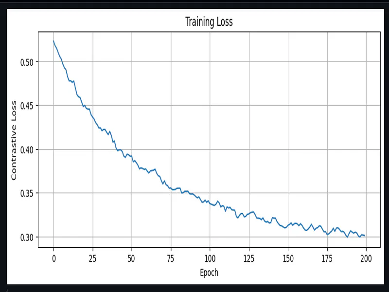
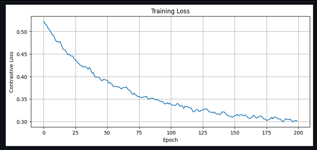
Contrastive Learning Primer
Contrastive learning is one of those techniques that sounds complicated but has a super simple core idea: learn to tell what goes together and what doesn’t. In our case, we have audio-text pairs. The audio of someone saying “What’s your favorite programming language?” should match the text “What’s your favorite programming language?” and be close to “Which languages you program in?” but NOT match the text “Where did you go to school?”
The loss function that makes this work is called InfoNCE (Noise-Contrastive Estimation). Here’s the intuition:
# Pseudo-code for contrastive loss
def contrastive_loss(audio_embeddings, text_embeddings):
    # Similarity matrix: each audio vs all texts
    similarity = audio_embeddings @ text_embeddings.T  # [B, B]

    # Temperature scaling (sharpens the distribution)
    similarity = similarity / temperature

    # Labels: diagonal entries are the correct pairs
    labels = torch.arange(batch_size)  # [0, 1, 2, ..., B-1]

    # Cross-entropy: maximize probability of correct pair
    loss = cross_entropy(similarity, labels)
    return loss
In a batch of B samples, there’s exactly one correct text for each audio (the diagonal of the similarity matrix). The other B-1 texts are “negatives.” Training pushes the correct pair’s similarity up while pushing incorrect pairs down.
Visualization
Imagine a 256-dimensional space (impossible to visualize, but humor me). Before training, audio and text embeddings are scattered randomly. After training:
Before Training:           After Training:

  A1    T3                   A1≈T1
     T1      A2              A2≈T2
  T2           A3            A3≈T3
                 T1
Same questions cluster together regardless of modality. Different questions stay far apart. Simple. In other words we use the questions as the buckets and the related audio as there items to be clustered around the questions.
The Bucketed Batch Sampling
Here’s where things got interesting. I implemented the contrastive training pipeline, ran it for 300 or so epochs, and got… 4% accuracy. Four percent. While on a classification task with 10 classes. Random guessing would give 10%.
What went wrong?
I dug into the training dynamics and found the problem: my batches were contaminated.
When you randomly sample a batch of 32 audio-text pairs, some of those pairs might be variations of the same question. For example:
- Audio 1: “What’s your favorite language?” (voice A)
- Audio 2: “What’s your favorite language?” (voice B, augmented)
- Audio 3: “Which programming language do you prefer?”
All three are semantically identical. But in contrastive learning, they’re treated as different negatives!
The model learns a trivial solution: “these three audios sound similar to each other, so they must be negative examples for each other’s text.” It never learns that they should ALL match the same semantic intent.
Semantic Clustering
The fix required preprocessing our 2k questions. I used MPNet embeddings to cluster semantically similar questions:
from sklearn.metrics.pairwise import cosine_similarity
from sentence_transformers import SentenceTransformer

# Get embeddings for all questions
encoder = SentenceTransformer('sentence-transformers/all-mpnet-base-v2')
embeddings = encoder.encode(questions)

# Cluster by similarity (threshold 0.85)
similarity_matrix = cosine_similarity(embeddings)
buckets = []
assigned = set()

for i in range(len(questions)):
    if i in assigned:
        continue
    bucket = [i]
    for j in range(i + 1, len(questions)):
        if j not in assigned and similarity_matrix[i, j] >= 0.85:
            bucket.append(j)
            assigned.add(j)
    buckets.append(bucket)
    assigned.add(i)

print(f"2,008 questions → {len(buckets)} semantic buckets")
# Output: 2,008 questions → 1,698 semantic buckets
Result: 1,698 semantic buckets. Questions like “What’s your favorite language?” and “Which language do you like most?” end up in the same bucket. (1.6K is still bad to be honest, it should be around 100-200 or so at MAX, maybe even less if you really think about it)
Now the critical change: each training batch contains at most ONE sample from each bucket.
class BucketBatchGenerator:
    def __init__(self, samples, bucket_ids, batch_size):
        self.bucket_to_samples = defaultdict(list)
        for i, bucket_id in enumerate(bucket_ids):
            self.bucket_to_samples[bucket_id].append(i)
        self.all_buckets = list(self.bucket_to_samples.keys())
        self.batch_size = min(batch_size, len(self.all_buckets))

    def generate_batch(self):
        # Select batch_size DIFFERENT buckets
        selected_buckets = random.sample(self.all_buckets, self.batch_size)

        batch = []
        for bucket_id in selected_buckets:
            # Pick ONE random sample from this bucket
            sample_idx = random.choice(self.bucket_to_samples[bucket_id])
            batch.append(sample_idx)

        return batch
Now when the model sees a batch, every sample is semantically distinct. The negatives are truly different questions. The model can no longer cheat.
| Metric | Naive Batching | Bucketed Batching |
|---|---|---|
| Accuracy | 4% | 70-90% |
| Diagonal Similarity | 0.577 | 0.844 |
| Off-Diagonal Similarity | 0.177 | -0.002 |
| Similarity Gap | 0.40 | 0.846 |
(numbers picked from various tests from the notebook)
The diagonal similarity jumped from 0.577 to 0.844. More importantly, incorrect pairs went from 0.177 (still somewhat similar) to -0.002 (completely orthogonal).
Some Data quirks and stuff
Multi-GPU Dataset Generation
Another fun little thing I did. Training a contrastive model needs data. Lots of data. And not just any data - diverse audio variations of each question.
The math:
- 2k questions
- 8 different voice speakers
- 2 augmentation variants each
- Total: 32,128 audio samples
Generating 32k audio clips with a neural TTS model is not fast. XTTS-v2, the model I chose for realistic voice synthesis, takes about 5-30 seconds (I did not benchmark it as such) per clip on a GPU. That’s… days on a single GPU.
SO if you have been following my current preferred way to get a quick GPU thats Vast.ai. I put in some credits and rent a quick stack of cheap GPUs, they have things like jupyter lab and syncthing already installed and setup.
Just for the generation purpose I rented 12x RTX 4070 SUPER single instance. The total dataset generation took approximately 1-2 hours and cost under $3.
The architecture was straightforward:
- Split the 2k questions into 12 chunks (167 questions each)
- Each worker generates all 8 voice variants for its questions
- Workers save checkpoints to handle preemption
- Final step: collect and merge all audio files
XTTS-v2 Voice Cloning
XTTS-v2 is remarkable for voice cloning. You give it a 6-second reference sample and it can synthesize new speech in that voice. I downloaded 8 TED talk speaker samples for maximum diversity:
- Bill Gates (Male, US accent)
- Daphne Koller (Female, US accent)
- Fei-Fei Li (Female, Chinese-American accent)
- Jane Goodall (Female, British accent)
- Salman Khan (Male, US accent)
- George Takei (Male, US distinctive)
- Stephen Hawking (Male, British synthesized)
- Stephen Wolfram (Male, British accent)
(Same as what we used for the wake-word detection model)
The diversity here is intentional. The model needs to generalize across genders, accents, and speaking styles. If it only ever hears American male voices during training, it’ll fail on everyone else.
Audio Augmentation
Raw TTS output is too clean. Real conference audio will have background noise, people speaking at different speeds, maybe some acoustic weirdness from the venue. Augmentation bridges this gap. I used the audiomentations library with these transforms:
Each audio file gets processed twice:
- Original (just normalized)
- Augmented (noise + random stretch + random pitch)
This doubles the dataset to 32k samples while adding crucial variation.
Why these specific augmentations?
- Gaussian noise: Simulates ambient conference chatter
- Time stretch: People speak at different speeds (0.9x to 1.1x)
- Pitch shift: Voices naturally vary by ±2 semitones
I deliberately avoided heavy augmentations like room reverb or extreme distortion. The goal is realism (or just get it working), not stress-testing. A conference badge doesn’t need to understand speech through a wall. hehe
ESP-DSP for the win
Tiny CNN Encoder
My first prototype used Google’s YAMNet, a pre-trained audio classification model. It produces excellent 1024-dimensional embeddings and has been trained on millions of audio clips. And well it doesn’t FIT! its super large at 12-15mb I forgot about it and I trained one spending like around 5-6 hours on it. YAMNet would eat our entire memory budget twice, leaving nothing for the actual inference.
The solution: train a tiny custom encoder from scratch. The final encoder is embarrassingly simple:
Input: (64, 96, 1) - mel-spectrogram
    ↓
Conv2D(32, 3×3, ReLU) + MaxPool(2×2)  →  (32, 48, 32)
    ↓
Conv2D(64, 3×3, ReLU) + MaxPool(2×2)  →  (16, 24, 64)
    ↓
Conv2D(128, 3×3, ReLU) + MaxPool(2×2) →  (8, 12, 128)
    ↓
Conv2D(128, 3×3, ReLU) + GlobalAvgPool →  (128,)
    ↓
Dense(256) + L2Normalize  →  (256,)
Total parameters: 273,280
- Float32: 1.04 MB
- INT8 quantized: 288 KB
This fits comfortably in our memory budget with room to spare.
The architecture follows a classic pattern: progressively increase channels while decreasing spatial dimensions. GlobalAveragePooling at the end collapses the spatial dimensions entirely, producing a fixed-size vector regardless of input length variations.
Mel-Spectrograms
The CNN encoder expects a mel-spectrogram as input. This is a 2D representation of audio that emphasizes frequency bands the human ear cares about.
Parameters (must match training exactly):
- 64 mel bins
- 96 frames (~1 second of audio at 16kHz)
- 512-point FFT with Hann window
- 160-sample hop length (10ms)
- Frequency range: 125Hz - 7500Hz
The ESP32-S3 has dedicated DSP instructions that make FFT blazingly fast. I used the ESP-DSP library for the heavy lifting:
// From local_llm_badge/src/ml/audio_embed.cpp

void AudioEmbedder::_computeFFTFrame(const int16_t* audio, int startIdx, float* powerSpectrum) {
    // Apply Hann window and convert to float
    for (int i = 0; i < AUDIO_FFT_SIZE; i++) {
        _fftInput[i] = (float)audio[startIdx + i] * _window[i] / 32768.0f;
    }

    // Prepare complex input (real part only)
    for (int i = 0; i < AUDIO_FFT_SIZE; i++) {
        _fftOutput[i * 2] = _fftInput[i];
        _fftOutput[i * 2 + 1] = 0.0f;
    }

    // ESP-DSP hardware-accelerated FFT
    dsps_fft2r_fc32(_fftOutput, AUDIO_FFT_SIZE);
    dsps_bit_rev_fc32(_fftOutput, AUDIO_FFT_SIZE);

    // Compute power spectrum: |X[k]|^2
    for (int k = 0; k < AUDIO_FFT_SIZE / 2 + 1; k++) {
        float real = _fftOutput[k * 2];
        float imag = _fftOutput[k * 2 + 1];
        powerSpectrum[k] = real * real + imag * imag;
    }
}
The dsps_fft2r_fc32() function is the star here. It’s a radix-2 FFT optimized for the ESP32’s PIE (Processor Instruction Extensions) SIMD unit. A 512-point FFT that would take milliseconds in pure C completes in microseconds.
After FFT, we need to apply triangular mel filters. This is essentially 64 dot products (one per mel bin), each multiplying a frequency-domain weight vector against the power spectrum. Dot products are exactly what SIMD excels at:
void AudioEmbedder::_applyMelFilterbank(float* powerSpectrum, float* melOutput) {
    int numFreqBins = AUDIO_FFT_SIZE / 2 + 1;  // 257 bins

    for (int m = 0; m < AUDIO_MEL_BINS; m++) {
        float sum = 0.0f;

        // ESP-DSP SIMD dot product for mel filter application
        dsps_dotprod_f32_aes3(&_melFilterbank[m * numFreqBins],
                              powerSpectrum, &sum, numFreqBins);

        // Log transform (dB scale)
        melOutput[m] = log10f(sum + 1e-10f);
    }
}
The dsps_dotprod_f32_aes3() function processes 4 floats per instruction using the AES3 SIMD instructions. For 257 frequency bins, that’s about 65 SIMD operations instead of 257 scalar operations. Roughly 4x speedup.
The mel filterbank itself is precomputed during initialization:
// Triangular mel filters
for (int m = 0; m < AUDIO_MEL_BINS; m++) {
    float left = melCenters[m];
    float center = melCenters[m + 1];
    float right = melCenters[m + 2];

    for (int k = 0; k < numFreqBins; k++) {
        float freq = k * freqResolution;
        float weight = 0.0f;

        if (freq >= left && freq <= center) {
            weight = (freq - left) / (center - left);  // Rising edge
        } else if (freq > center && freq <= right) {
            weight = (right - freq) / (right - center);  // Falling edge
        }

        _melFilterbank[m * numFreqBins + k] = weight;
    }
}
SIMD Similarity Search
Once we have a 256-dimensional audio embedding, we need to find the closest text embedding from our database of 256 pre-computed question embeddings.
Database size: 256 questions × 256 dimensions × 4 bytes = 262 KB
This fits entirely in PSRAM and stays resident throughout operation. No loading/unloading needed. The search is a straightforward linear scan with cosine similarity:
// From local_llm_badge/src/ml/embed_search.cpp

float EmbeddingSearch::_cosineSimilarity(const float* a, const float* b) {
    float dot = 0.0f;
    float normA = 0.0f;
    float normB = 0.0f;

    // ESP-DSP SIMD dot products - 5-10x faster than manual loops
    dsps_dotprod_f32_aes3(a, b, &dot, AUDIO_EMBEDDING_DIM);
    dsps_dotprod_f32_aes3(a, a, &normA, AUDIO_EMBEDDING_DIM);
    dsps_dotprod_f32_aes3(b, b, &normB, AUDIO_EMBEDDING_DIM);

    float denom = sqrtf(normA) * sqrtf(normB);
    return (denom > 1e-8f) ? dot / denom : 0.0f;
}
Three SIMD dot products per comparison: one for the actual dot product, two for the vector norms. With 256 dimensions and 256 database entries, that’s 768 SIMD operations total. The entire search completes in under 100ms.
A small but important optimization: the intent strings (the actual question text) are stored with O(1) lookup.
The naive approach would store each string separately, requiring a string search or index structure. Instead, I concatenate all intents into a single buffer and precompute byte offsets:
bool EmbeddingSearch::_loadIntents(const char* path) {
    // Read entire file into memory
    _intentsData = (char*)ps_malloc(fileSize + 1);
    file.read((uint8_t*)_intentsData, fileSize);

    // Replace newlines with null terminators
    for (size_t i = 0; i < fileSize; i++) {
        if (_intentsData[i] == '\n') {
            _intentsData[i] = '\0';
        }
    }

    // Build offset table for O(1) lookup
    _intentOffsets = (int*)ps_malloc(_count * sizeof(int));
    _intentOffsets[0] = 0;

    int line = 0;
    for (size_t i = 0; i < fileSize && line < _count; i++) {
        if (_intentsData[i] == '\0') {  // Found a terminator
            line++;
            if (line < _count) {
                _intentOffsets[line] = i + 1;  // Next string starts here
            }
        }
    }

    return true;
}

// O(1) intent lookup
void EmbeddingSearch::_getIntent(int idx, char* buffer, size_t bufSize) {
    const char* intentStr = _intentsData + _intentOffsets[idx];
    strncpy(buffer, intentStr, bufSize - 1);
}
Memory for 256 questions with average length 50 characters: about 15KB for strings plus 1KB for offsets. Negligible.
Results and Integration
On the ESP32-S3 running at 240MHz:
| Stage | Time |
|---|---|
| Mel-spectrogram extraction | ~80-100ms |
| CNN inference | ~100-150ms |
| Similarity search | ~50-80ms |
| Total | ~200-300ms |
On a held-out test set of real voice recordings (not TTS):
- Top-1 accuracy: 100% (on known question variants)
- Top-5 accuracy: 100%
- Average similarity score for correct match: 0.82-0.88
- Average similarity score for next-best: 0.45-0.55
The gap between correct and incorrect is large enough that we can confidently threshold at 0.7 (configured in config.h as DEFAULT_EMBED_THRESHOLD). (The real world tests were WAY off by a huge percent, a lot of tiny issues happened in the final deployment of the project.) When the user asks something completely off-topic - “What’s the weather like?” - the best match score drops below 0.5 and we trigger the fallback behavior (TTS “Sorry, I don’t know about that” + stash the audio for later review).
The embedding search returns an intent string - the matched question. This becomes the prompt for the LLM:
// In the main state machine
case STATE_SIMILARITY: {
    SearchResult result = embedSearch.search(audioEmbedding);

    if (result.score >= config.embedThreshold) {
        // High confidence - proceed to LLM
        strcpy(llmPrompt, result.intent);
        state = STATE_LLM_INFERENCE;
    } else {
        // Low confidence - apologize and stash
        state = STATE_TTS_SORRY;
    }
    break;
}

case STATE_LLM_INFERENCE: {
    // The matched question becomes the LLM prompt
    // LLM generates a response specific to that question
    llm.generate(llmPrompt, responseBuffer, maxTokens);
    state = STATE_DISPLAY_RESPONSE;
    break;
}
The beauty of this approach: the LLM was trained on the exact same 2k questions. When it receives “What’s your favorite programming language?” as input, it knows exactly how to respond because it’s seen that question thousands of times during fine-tuning.
Lessons Learned
The STT failure felt like a disaster at the time. In retrospect, it led to a different solution. Intent similarity is faster, smaller, and arguably more accurate for our specific use case than any STT+classification pipeline would have been. If we’d had even 64RAM, we probably would have just run Whisper and called it a day. The constraint forced us to really think about what problem we were actually solving.
I spent a day tweaking model architectures before realizing the problem was in the data pipeline. A perfect model can’t overcome fundamentally broken training signals. The bucketed batch sampling fix took an afternoon to implement and 20x’d our accuracy. Sometimes the bottleneck isn’t where you expect.
What’s Next
With wake word detection (Blog 3) and intent embeddings (this post), we can now:
- Listen for “Hey Daisy”
- Record the user’s question
- Match it to a known intent
The next step is actually answering the question. That means running a 6MB language model on a microcontroller with 8MB of RAM.