Training Custom Wake Word for ESP32

In the first blog of this series, we got MJPEG video playing on our ESP32-S3 badge with gyroscope-based rotation. Then in the second blog, we dove deep into running a tiny LLM on the same chip. Next is developing an interface to interact with it. Since its a badge I didn’t want buttons and stuff that people would have to press to input into the LLM, therefore introducing a little wake word “Hey Daisy” to capture the audio and then make it text and then feed it to the LLM. But this blog we are only going to focus on the wake word part. We custom trained one for this project.

Lookback

If you’ve ever said “Hey Siri” or “OK Google,” you’ve used wake word detection. I set my alarms and all kinds of things using my Google assistant, its addicting. So yeah the idea is simple: instead of requiring a button press, the device listens constantly for a specific trigger phrase. Everything else gets ignored.

The alternative was push-to-talk, which works fine but feels clunky for a conference badge. (Truth to be told my conference badge was still clunky after we put together everything) Imagine walking up to someone, reaching for a button, pressing it, then speaking. The whole interaction becomes awkward. With wake word detection, you just say “Hey Daisy, tell me about yourself” and the badge responds. Much more natural.

Now heres the challenging part: wake word detection has to run constantly. Unlike the LLM that only fires when needed, the wake word model runs on every audio frame. That means it needs to be tiny, fast, and accurate. We’re talking about a model that can process audio in real-time.

The MicroWakeWord Framework

After researching options, I settled on microWakeWord by Kevin Ahrendt. It’s specifically designed for microcontrollers, with training pipelines that produce TFLite models optimized for streaming inference.

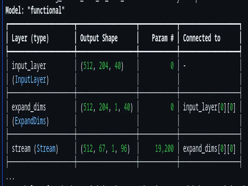
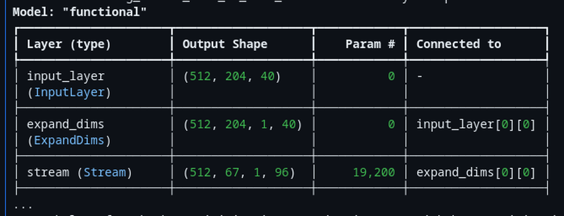
The architecture is based on MixNet, which is essentially a MobileNet variant with mixed depthwise convolutions. What makes it special for wake word detection is the streaming design - the model maintains internal state between frames, processing one small chunk of audio at a time rather than requiring the entire utterance upfront.

Here’s what the training config looks like for our model:

# Model architecture

# Number of output channels for pointwise (1x1) convolutions in each block
pointwise_filters = '192,192,192,192'

# How many times to repeat each MixNet block
repeat_in_block = '1,1,1,1'

# Mixed depthwise convolution kernel sizes per block - different sizes capture different temporal patterns
mixconv_kernel_sizes = '[5], [7,11], [9,15], [23]'

# Temporal stride - how many frames to skip between outputs (controls output length)
stride = 3

# Number of filters in the first convolution layer
first_conv_filters = 96

# Kernel size for the first convolution layer
first_conv_kernel_size = 5

The resulting model is around 200kb, which might sound big or tiny depending on what background you come from. Very tiny for someone who might be developing stuff for PCs and big machine with plenty RAM, but quite big if you are someone already working in the embedded space. It includes all the state needed for streaming inference. The model takes in 40-bin log-mel spectrogram features (3 frames at a time) and outputs a single probability: how likely is it that the wake word was just spoken? (OR maybe the model was just too small and I super over-fit it with all the crazy amount of training data, keeping these fixes for next time)

I’ll be honest - I don’t fully understand all the MixNet architectural choices. Claude helped me understand that the mixed kernel sizes (5, 7, 11, 9, 15, 23) allow the model to capture both fine-grained phonetic details and longer temporal patterns. But the math behind why these specific numbers work? Still a bit fuzzy to me. What I do know is that it works, and the model size fits our constraints. Thats pretty much what I needed to get done when I was working on this project in a tight deadline.

Generating the Training Data

This is where things got interesting. Training a wake word detector requires thousands of positive samples (people saying “Hey Daisy”) and even more negative samples (everything else). Recording real people saying the phrase thousands of times wasn’t practical, so we went full synthetic.

Phonetic Variations

First, I created 20 different phonetic variations of “Hey Daisy”:

PHONETIC_VARIATIONS = [
    "Hey Daisy ", "hey Daisy ", "hey daisy ",
    "Hey Daisy. ", "Hey Daisy! ",
    "hey day zee ", "hey day-zee ", "hey daisee ",
    "hey daysy ", "hey daezy ",
    "hay daisy ", "hay Daisy ",
    "HEY Daisy ", "hey DAISY ", "HEY DAISY ",
    "hey daisy? ", "heyyy daisy ",
    "hey daizy ", "hey dayzie ", "hey dazey ",
]

Why so many variations? Different Text-to-speech models interpret text differently based on capitalization, punctuation, and spelling. “HEY DAISY” sounds more emphatic than “hey daisy”. The trailing space matters too - without it, some TTS engines produce clipped audio, that space gives it a pause like feeling.

Piper TTS for Volume

For the bulk of our samples, we used Piper TTS with the LibriTTS medium model. It’s fast and can generate diverse voices:

python3 generate_samples.py "Hey Daisy " \
    --max-samples 100 \
    --model en_US-libritts_r-medium.pt

100 samples per variation = 2,000 Piper samples total.

XTTS-v2 for Realism

Piper is great for volume, but the voices can sound synthetic or made up like. For more realistic samples, we used XTTS-v2 with voice cloning from TED speaker recordings:

TED_SPEAKERS = ['BillGates', 'DaphneKoller', 'FeiFeiLi', 'GeorgeTakei',
                'JaneGoodall', 'SalmanKhan', 'StephenHawking', 'StephenWolfram']

The speaker samples are from audio-samples.github.io, which hosts freely available TED speaker voice clips perfect for voice cloning.

8 speakers x 10 voice samples each x 20 variations = 1,600 XTTS samples.

Combined total: 3,600 positive samples of “Hey Daisy” in various voices, accents, and intonations.

The full training notebook was attached in the top if you want to see the gory details.

Confusable Negatives

I learned something the hard way. So during my initial batch of experiments I trained multiple models of different architectures, sizes and data sizes. After all the training and all I ran it on my ESP and during testing I realized a big flaw: it kept triggering on phrases that weren’t “Hey Daisy.”

“Hey crazy!” - TRIGGERED. “Hey lazy!” - TRIGGERED. “Hey baby!” - TRIGGERED. “Daisy” alone - TRIGGERED. Just “Hey” - TRIGGERED.

The model was picking up on phonetic similarity without learning to reject near-misses. The generic “speech” and “no speech” negative samples from microWakeWord’s default dataset weren’t enough. They taught the model to distinguish wake word from silence or random chatter, but not from similar phrases. And considering that “Daisy” was not really a very unique sounding word and that it had a lot of similarity with many other words, it would be even more difficult for the model to learn the exact sound of it.

The solution? Confusable negatives - explicit samples of what the model should NOT trigger on, weighted heavily during training.

CONFUSABLE_NEGATIVES = [
    # Partials (most important!)
    "Hey ", "hey ", "HEY ", "hay ",
    "Daisy ", "daisy ", "DAISY ", "daisee ", "daysy ", "day zee ",

    # Similar to "Daisy"
    "crazy ", "lazy ", "hazy ", "mazy ",
    "Tracy ", "Stacy ", "Gracie ", "Lacey ", "Macy ", "Casey ",
    "racy ", "spacey ",

    # Similar phrases
    "hey crazy ", "hey lazy ", "hey Tracy ", "hey Stacy ",
    "hey baby ", "hey lady ", "hey maybe ", "hey safety ",
    "say daisy ", "pay daisy ", "play daisy ", "stay daisy ",

    # Rhyming words
    "haze ", "days ", "daze ", "phase ", "craze ",
    "maze ", "blaze ", "gaze ", "raise ", "praise ",

    # Common "hey" phrases
    "hey there ", "hey you ", "hey what ", "hey how ",
    "hey wait ", "hey look ", "hey come ", "hey stop ",

    # Other flower names
    "hey Rose ", "hey Lily ", "hey Violet ", "hey Iris ", "hey Poppy ",
]

That’s 63 confusable phrases. At 50 Piper samples per phrase, we generated 3,150 confusable negative samples.

The key is the sampling weight during training:

{
    'truth': False,  # These are NEGATIVES
    'sampling_weight': 15.0,  # HIGH weight - prioritize learning these!
    'penalty_weight': 2.0    # Extra penalty for false positives
}

A sampling weight of 15.0 means confusable negatives appear 15x more often during training than their natural frequency would suggest. The model sees “hey lazy” over and over, each time learning “this is NOT the wake word.”

After retraining with confusable negatives, the false positive rate dropped dramatically. “Hey crazy” no longer triggers. “Hey Daisy” still does. More of less success. (There were more harsh learning that I will share later)

Audio Augmentation Pipeline

Real-world audio is messy. Conference halls have background chatter. Someone might mumble. There might be music playing. To make our model robust, we augmented the training data heavily.

augmentation = Augmentation(
    augmentation_probabilities={
        "SevenBandParametricEQ": 0.1,
        "TanhDistortion": 0.1,
        "PitchShift": 0.1,
        "BandStopFilter": 0.1,
        "AddColorNoise": 0.1,
        "AddBackgroundNoise": 0.75,  # 75% of samples get background noise
        "Gain": 1.0,                  # Always vary volume
        "RIR": 0.5,                   # 50% get room impulse response
    },
    impulse_paths=['/path/to/mit_ir/Audio'],  # MIT impulse database
    background_paths=['/path/to/audioset'],   # AudioSet background noises
)

Background Noise Injection (75% probability): We downloaded 500 samples from AudioSet - everything from crowd noise to machinery to music. Adding these as background teaches the model to pick out “Hey Daisy” from a noisy environment.

Room Impulse Response Convolution (50%): MIT provides a database of impulse responses recorded in various rooms. Convolving our dry TTS audio with these makes it sound like it was recorded in an actual room with reflections and reverb. This is crucial because the badge will be used in conference halls, not anechoic chambers.

SpecAugment Its a technique from Google that masks random time and frequency regions of the spectrogram:

'time_mask_max_size': [10],   # Up to 10 frames
'time_mask_count': [2],        # Two time masks
'freq_mask_max_size': [3],     # Up to 3 frequency bins
'freq_mask_count': [2],        # Two frequency masks

This prevents the model from over-relying on any specific time or frequency pattern.

With augmentation, our 3,600 positive samples become 288,000 training spectrograms (10x repetition with different augmentations). The confusable negatives become 126,000 spectrograms (5x repetition). I really think I overdid it, next time when I work on this I will try to learn and understand the underlying stuff more carefully and make the training data with more consciousness decisions. It was a fun thing to begin with.

Feature Extraction

Before audio hits the model, it needs to be converted to spectrograms. We use the TensorFlow Lite Microfrontend library, which is designed specifically for embedded devices.

The feature extraction config, defined in local_llm_badge/src/audio/mic_stream.h:

#define FEATURE_WINDOW_MS   30   // 30ms analysis window
#define FEATURE_STRIDE_MS   10   // 10ms between frames (67% overlap)
#define FEATURE_BINS        40   // 40 mel-frequency bins
#define FEATURE_FRAMES      3    // Model input: 3 frames at a time

The frontend does several things:

1. Mel filterbank: Converts the raw FFT (Fast Fourier Transform) output to mel-frequency bins. The mel scale is a perceptual scale where equal distances correspond to equal perceived pitch differences - it mimics how human ears perceive sound frequencies (we’re more sensitive to differences in lower frequencies than higher ones)
2. PCAN gain control: Adaptive gain that normalizes volume, making the model robust to quiet or loud speech
3. Noise reduction: Smooths and suppresses background noise

From local_llm_badge/src/audio/mic_stream.cpp:

bool MicStream::_initFrontend() {
    FrontendConfig frontend_config;
    frontend_config.window.size_ms = FEATURE_WINDOW_MS;
    frontend_config.window.step_size_ms = FEATURE_STRIDE_MS;
    frontend_config.filterbank.num_channels = FEATURE_BINS;
    frontend_config.filterbank.lower_band_limit = 125.0f;
    frontend_config.filterbank.upper_band_limit = 7500.0f;
    frontend_config.noise_reduction.smoothing_bits = 10;
    frontend_config.noise_reduction.even_smoothing = 0.025f;
    frontend_config.noise_reduction.odd_smoothing = 0.06f;
    frontend_config.noise_reduction.min_signal_remaining = 0.05f;
    frontend_config.pcan_gain_control.enable_pcan = 1;
    frontend_config.pcan_gain_control.strength = 0.95f;
    frontend_config.pcan_gain_control.offset = 80.0f;
    frontend_config.pcan_gain_control.gain_bits = 21;
    frontend_config.log_scale.enable_log = 1;
    frontend_config.log_scale.scale_shift = 6;

    return FrontendPopulateState(&frontend_config, _frontendState, SAMPLE_RATE);
}

The PCAN gain control is particularly important. Without it, someone whispering “Hey Daisy” from far away would produce much smaller values than someone shouting it nearby. PCAN normalizes both to similar magnitudes, improving detection at various volumes. (But later in the end during the complete integration phase which is a later blog, I messed this up I think, this gain control thing or something was missing up the initial 1-2 seconds of the audio that was being recorded right after the wake word. I didn’t properly tune these values for my use case, most of it AI generated as is used.)

On-Device Inference with EdgeNeuron

I had a hard requirement for the entire project, I was NOT going to setup ESP-IDF or PlatformIO in my vscode to compile and do all the programs and stuff. I wanted to stick with Arduino IDE for the sake of simplicity of setup and usage. So a proper TFLite library running seemed a bit challenging, I tried a lot of different approaches here, none really panned out, in most cases some feature A would work and then feature B would fail and so on. It was getting so annoying that I was on the verge of giving up BUT during my deep internet searches I came across the EdgeNeuron library, which bundles TensorFlow Lite Micro with the microfrontend. (The initial build took enough time, but the subsequent builds were pretty normal and usual speed of around 5-10 seconds or so)

The Dual-Arena Setup

Streaming models need two memory regions:

• Tensor arena (502KB): For input/output tensors and intermediate activations
• Variable arena (52KB): For persistent state between frames

From local_llm_badge/src/ml/wake_word.h:

static constexpr size_t TENSOR_ARENA_SIZE = 502000;
static constexpr size_t VAR_ARENA_SIZE = 52000;
static constexpr int MAX_RESOURCE_VARS = 100;

Placement New for Interpreter Reset

Here’s a pattern I learned during debugging. When you need to reload a model (say, after switching between wake word and audio embedding models), you can’t just create a new interpreter on embedded systems. The problem is memory fragmentation - if you allocate a new interpreter with regular new, the old interpreter’s memory might not be freed contiguously, leaving holes in your heap. On a microcontroller with limited RAM, these holes can quickly add up and cause allocation failures. The solution is C++ placement new:

// Placement new resets interpreter state without reallocation
static uint8_t interpreterBuffer[sizeof(tflite::MicroInterpreter)] __attribute__((aligned(16)));
_interpreter = new (interpreterBuffer) tflite::MicroInterpreter(
    model, resolver, _tensorArena, TENSOR_ARENA_SIZE, _resourceVars);

This constructs a new interpreter object in a pre-allocated buffer, ensuring the destructor of the old interpreter runs first. It’s critical for avoiding memory fragmentation when loading/unloading models.

Quantization-Aware Feature Conversion

The model expects int8 input, but our microfrontend produces uint16 values. The conversion needs to match what was done during training:

if (_inputTensor->type == kTfLiteInt8) {
    int8_t* input_data = _inputTensor->data.int8;
    for (int i = 0; i < total_features; i++) {
        // Convert uint16 features to int8 range [-128, 127]
        int32_t scaled = ((int32_t)features[i] * 256 + 333) / 666 - 128;
        input_data[i] = constrain(scaled, -128, 127);
    }
}

Getting this scaling wrong was a source of many hours of debugging. The model would produce garbage outputs until we matched the exact quantization math from training. Claude helped me trace through the microWakeWord Python code to find the right formula. (Like I said once am no genius or expert in any of this, all I know if to read and debug and guess problems. Claude pretty much helps with the rest.)

Sliding Window Detection

A single inference gives us a probability. But one high probability could be noise. We need temporal consistency - the probability should stay high across multiple frames when the wake word is actually spoken.

The detection logic from local_llm_badge/src/ml/wake_word.cpp:

bool WakeWordDetector::detect(const uint16_t* features) {
    if (!_loaded) return false;

    // Run inference
    float prob = _runInference(features);
    _lastProbability = prob;

    // Update sliding window
    _probabilityWindow[_windowPos] = prob;
    _windowPos = (_windowPos + 1) % _config.sliding_window_size;

    if (_windowPos == 0) {
        _windowFilled = true;
    }

    // Need full window before detection
    if (!_windowFilled) {
        return false;
    }

    // Check cooldown
    if (millis() - _lastDetectionMs < (unsigned long)_config.cooldown_ms) {
        return false;
    }

    // Calculate average and count high frames
    float avg = 0.0f;
    int high_frames = 0;
    for (int i = 0; i < _config.sliding_window_size; i++) {
        avg += _probabilityWindow[i];
        if (_probabilityWindow[i] >= _config.min_frame_prob) {
            high_frames++;
        }
    }
    avg /= _config.sliding_window_size;

    // Detection criteria: avg >= 0.5 AND >= 6 frames > 0.5
    if (avg >= _config.probability_cutoff && high_frames >= _config.min_high_frames) {
        _lastDetectionMs = millis();
        _resetWindow();
        return true;
    }

    return false;
}

The detection requires BOTH conditions:

1. Average probability across 10 frames >= 0.5
2. At least 6 of those 10 frames have probability > 0.5

This prevents false triggers from a single spike while still allowing quick detection when the wake word is genuinely spoken.

Cooldown Mechanism

“re-triggering” is something that kept on happening quite a lot, so we added a little cooldown period to prevent it. The default is 1500ms (1.5 seconds). This gives time for the user to start speaking their actual question before the badge could potentially re-trigger on echo or feedback.

Runtime Configuration

All the detection parameters are configurable via JSON on the SD card, meaning you can tune the sensitivity without recompiling:

{
  "type": "micro",
  "wake_word": "Hey Daisy",
  "model": "hey_daisy.tflite",
  "version": 1,
  "micro": {
    "probability_cutoff": 0.5,
    "sliding_window_average_size": 10,
    "min_high_frames": 6,
    "min_frame_prob": 0.5,
    "cooldown_ms": 1500
  }
}

This lives at /models/hey_daisy.json on the SD card. If you’re getting too many false positives at a conference, bump probability_cutoff to 0.6 or 0.7. Too many missed detections? Lower min_high_frames to 4 or 5.

Results and Lessons Learned

After all that work, here’s where we ended up:

Performance Numbers

• Model size: ~130kb TFLite (quantized int8)
• Inference time: ~50ms per frame
• True positive rate: ~85% in quiet environments, ~71% with moderate background noise

1. Wake word detection is harder than it looks. It’s not just “detect a phrase” - it’s “detect THIS phrase and ONLY this phrase, even when something very similar is said.”
2. Streaming models are tricky. The state management, arena sizing, and proper interpreter reinitialization all have gotchas. The placement new pattern for interpreter reset was not obvious.

What’s Next

The wake word detector triggers. Great. But then what? The badge needs to understand what you said after the trigger phrase. That’s where things get really interesting - and where we hit the limits of what fits in 8MB of PSRAM. Spoiler: we couldn’t fit any speech-to-text model, so we invented a workaround using audio embeddings and similarity search.

But that’s a story for the next blog.